
Introduction
When you want to compare the average outcome of two separate groups, you need a method that distinguishes real differences from random variation. The Independent Samples T-Test (also called the two-sample t-test) is one of the most widely used statistical tools for this purpose. It helps you test whether two population means are likely to be different based on sample data. In applied analytics, this shows up in A/B testing, product experiments, policy evaluations, and quality control. For learners in a data scientist course, mastering this test is essential because it builds a strong foundation for experimental reasoning and model validation.
When to Use an Independent Samples T-Test
You use an independent samples t-test when:
- You have two groups that are independent (no overlap in participants or observations).
- You want to compare the mean of a continuous variable (for example, time on site, revenue, test scores, blood pressure).
- Your goal is to determine whether the observed difference in sample means is statistically meaningful.
Common examples include:
- Comparing average conversion rates (or average basket value) between two marketing campaigns.
- Comparing average customer satisfaction scores between two service centres.
- Comparing average defect rates between two manufacturing lines (if data is continuous or can be treated as such).
If the same subjects are measured twice (before and after, or repeated measures), you would use a paired t-test instead. Understanding this distinction is frequently emphasised in a data science course in Mumbai because it affects how you interpret evidence from business experiments.
Hypotheses and the Core Idea
The t-test is built around hypothesis testing:
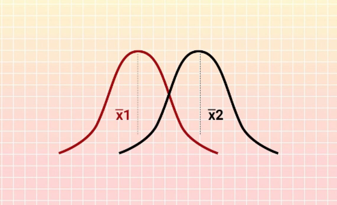
- Null hypothesis (H₀): The population means are equal (μ₁ = μ₂).
- Alternative hypothesis (H₁): The population means are not equal (μ₁ ≠ μ₂).
You can also run one-sided tests when you have a directional expectation, such as μ₁ > μ₂. However, one-sided tests should be chosen before analysing the data, not after.
The test calculates a t-statistic, which reflects how large the mean difference is relative to the variability in the data. A bigger absolute t-statistic indicates the difference is less likely to be explained by chance alone.
Assumptions You Must Check
The independent samples t-test works best when key assumptions are reasonably satisfied. In many real datasets, these assumptions are approximations, so it helps to understand what matters most.
- Independence of observations
The two samples must not influence each other. This is the most important assumption. If independence fails, the p-values can become misleading. - Approximate normality
Each group’s outcome should be roughly normally distributed, especially for small sample sizes. With moderate to large samples, the Central Limit Theorem often makes the t-test fairly robust. - Homogeneity of variances (equal variances assumption)
Standard t-tests assume both groups have the same variance. If one group is much more variable than the other, you should use Welch’s t-test, which adjusts degrees of freedom and is commonly recommended as a safer default.
In practice, analysts often use diagnostic checks:
- Visual checks (histograms, box plots)
- Variance comparison (for example, Levene’s test)
- Reviewing whether sample sizes are similar
How to Run and Interpret the Test
A typical workflow looks like this:
- State hypotheses and choose significance level (α)
Common values are 0.05 or 0.01. - Compute sample means and standard deviations
The mean difference is the practical quantity of interest. - Compute the t-statistic and p-value
The p-value indicates how consistent your data is with the null hypothesis. - Make a decision
- If p ≤ α: reject H₀ (evidence suggests the means differ).
- If p > α: fail to reject H₀ (insufficient evidence of difference).
A crucial point: “Failing to reject” does not prove the means are equal. It may simply mean you do not have enough data to detect a difference.
Effect Size and Confidence Intervals
Statistical significance alone is not enough. A small difference can be statistically significant in large samples but irrelevant in practice. That is why you should report:
- Confidence interval (CI) for the mean difference
This provides a range of plausible values for the true difference. If the CI excludes zero, it aligns with a statistically significant result. - Effect size (Cohen’s d)
Cohen’s d measures the mean difference relative to pooled variability. It helps compare results across different contexts. As rough guidance, 0.2 is small, 0.5 medium, and 0.8 large, but interpretation depends on the domain.
In business settings, a confidence interval combined with a practical threshold (for example, “we need at least a 2% improvement”) leads to clearer decisions than p-values alone.
Common Pitfalls and How to Avoid Them
- Using a t-test for non-independent groups: This often happens when samples overlap or when data is paired.
- Ignoring unequal variances: Welch’s t-test is typically a better default than assuming equal variances.
- Over-focusing on p-values: Always examine the effect size and confidence interval.
- Multiple comparisons without correction: If you test many metrics or segments, false positives increase. Consider corrections or pre-registered hypotheses.
These pitfalls are frequently addressed in a data scientist course because they can directly cause incorrect business conclusions.
Conclusion
The independent samples t-test is a core tool for comparing the means of two independent groups. It provides a structured way to test whether an observed difference is likely to reflect a real population effect rather than random sampling noise. To use it responsibly, confirm independence, consider variance differences (often using Welch’s t-test), and report confidence intervals and effect sizes alongside p-values. With these practices, the t-test becomes a reliable method for evidence-based decisions in experimentation and analytics-skills that remain central to a data science course in Mumbai and modern data-driven work.
Business Name: ExcelR- Data Science, Data Analytics, Business Analyst Course Training Mumbai
Address: Unit no. 302, 03rd Floor, Ashok Premises, Old Nagardas Rd, Nicolas Wadi Rd, Mogra Village, Gundavali Gaothan, Andheri E, Mumbai, Maharashtra 400069, Phone: 09108238354, Email: enquiry@excelr.com.